Introduction
Polyploidy refers to the presence of more than two sets of chromosomes within a single organism (Mason 2017). Polyploidy plays important roles in agriculture (Hilu 1993), species evolution (Otto and Whitton 2000; Joly et al. 2006; Wendel 2000), medicine (Coward and Harding 2014), among other fields. The research on polyploids is thus extensive. Several agricultural crops, such as wheat, soybean, potatoes, sugarcane, and cotton are polyploids (Hilu 1993), and polyploidy plays an important role on plant evolution (Otto and Whitton 2000). Polyploidization is also a property of some cancerous cells (Coward and Harding 2014). Therefore, studying polyploids is of great significance.
Polyploids are often divided into two categories based on their evolutionary histories — allopolyploids and autopolyploids (Cao, Osborn, and Doerge 2004). Autopolyploids arise from whole genome duplications within a single species. Allopolyploids arise by hybridization between species yielding polyploidization (Bourke et al. 2017). Chromosomes are also divided into two categories. Two chromosomes that arise from the same species are called homologues. Two chromosomes that arise from separate species are said to be homoeologues.
Allopolyploids and autopolyploids are often distinguishable by their meiotic behavior, which exhibits greater complexity than in diploids. Meiosis is an elementary process in biology (Voorrips and Maliepaard 2012), which allows parents to send their genetic materials to the next generation. There are many steps to meiosis, but we will focus on the pairing behavior during prophase I. During prophase I, the nucleoli and nuclear envelop disappear, hom(oe)ologous chromosomes pair and exchange genetic material. In allopolyploids, homologous chromosomes always pair with each other during prophase I. In autopolyploids, hom(oe)ologous chromosomes randomly pair together with no preference.
The definition of autopolyploidy and allopolyploidy based on the evolutionary background depends on arbitrary thresholds of evolutionary relatedness of homoeologues. Characterizing meiotic behavior requires no such thresholds and so researchers have also suggested defining ploidy by their meiotic behavior. However, unlike in diploids, where a parent sends one copy to each offspring, in polyploids there is greater diversity in the behavior of gametic transmission. For example, in tetraploids (individuals with four copies of their genome) there are \(\binom{4}{2}/2!\) = 3 ways that gametes can pair during meiosis. Therefore, there are many complications in estimating meiotic behavior. A complication that arises in distinguishing between ploidy types is that some pairing configurations are more common than other (Sybenga 1994). In a polyploid the given chromosomes may be completely homologues or there may be two slightly different types (homoeologues) present that pair more easily with their own type than with the other (Voorrips and Maliepaard 2012). The degree of preferential pairing may vary from 0% (fully random pairing, as in autopolyploids where the four copies of a chromosome are completely homologous) to 100% (the homoeologues pair exclusively with their own type, as in allopolyploids). Thus, intermediate forms with partially preferential pairing may occur. Therefore, based on pairing behavior in meiosis, there are three pairing behaviors: autopolyploids, allopolyploids, and intermediate levels of preferential pairing (Bourke et al. 2017).
Preferential pairing has been estimated in several ways. Ancestral origin frequencies are used to infer preferential pairing rates (Sybenga 1994). The method of haplotype reconstruction, provided in TetraOrigin, consists of multilocus parental linkage phasing and subsequent ancestral inference from SNP dosage data (Zheng et al. 2016). Preferential pairing can also be estimated by examining repulsion‐phase linkage patterns (Bourke et al. 2017).
Unfortunately, none of the above methods directly use genotype data, a common form of data in the modern sequencing age. For many types of data, the dosage of alleles are available at individual loci, but the phased configuration of these alleles are not known. These data often result from next-generation sequencing technologies that are then genotyped using genotyping software (Gerard et al. 2018; Gerard and Ferrão 2019; Clark, Lipka, and Sacks 2019; Blischak, Kubatko, and Wolfe 2018; Voorrips, Gort, and Vosman 2011). We use genotype data with F1 population (full-sib progeny of two parents) directly to analysis preferential pairing. Throughout, we assume that we are dealing with a tetraploid population and leave higher ploidy levels for future work. Therefore, In this thesis, we wish to distinguish between the types of ploidy and to estimate the strength of preferential pairing in polyploids from genotype data with F1 population directly.
In this thesis, we will use F1 population in genotype data, which consists of full-sib progeny of two parents. In an F1 population, each individual is the result of two meiotic divisions from each parent. We thus have replications of the meiotic behavior from each parent. We begin by providing a way to estimate preferential pairing at each locus from parents’ and progenies’ genotype. Due to the unidentifiability of which chromosomes contain which alleles, we provide a way based on clustering to identify this and estimate interpretable parameters. At last, through a simulation study, we demonstrate that our work can distinguish between the types of ploidy from genotype data directly.
The following is the outline of our paper. In Section 2.1, we provide a way to estimate preferential pairing at each locus using just genotype data. In Section 2.2, we provide a way to identify the parameterization and estimate interpretable parameters using model-based clustering. We demonstrate, through simulations, in Section 3.1 that we can accurately estimate the levels of preferential pairing at each locus through maximum likelihood estimation. We demonstrate in Section 3.2 that we can accurately distinguish between autopolyploidy and intermediate levels of polyploidy. However, we note that accurately detecting allopolyploidy is difficult. We conclude with a discussion in Chapter 4 .
Methods
Estimating Preferential Pairing using Maximum Likelihood Estimation
In this section, we will introduce a method to estimate preferential pairing from genotype data. We will now describe the data under consideration. We assume that we are working with an F1 population (a biparental cross) which is common in breeding populations (Sybenga 1994). An F1 population consists of parents and offspring. We assume that we have genotype data from each parent and each offspring. Genotype data consists of an integer \(\{0, 1, \ldots,K\}\) of the number of reference alleles an individual contains at a bi-allelic locus. We will denote the reference allele by and the alternative allele by . We denote the ploidy by \(K\), which we assume to be the same for all individuals. In our research, we are interested the pairing behavior in tetraploids (\(K = 4\)). For convenience, we have summarized all the parameters we used in Table 1.
| Parameter | Means |
|---|---|
| \(K\) | The ploidy of the species. In our model, we assume all individuals are tetraploid (i.e. \(K = 4\)). |
| \(\ell_j\) | The genotype of parent \(j\), which is defined as the dosage of A’s in parent \(j\)’s genome. |
| \(\boldsymbol m_{ij}\) | Pairing configuration of a parent for a child \(i\). \(\boldsymbol m_{ij}=(m_{1ij}, m_{2ij}, m_{3ij})\) |
| \(m_{1ij}\) | The number of copies of “aa” from parent \(j\) |
| \(m_{2ij}\) | The number of copies of “Aa” from parent \(j\) |
| \(m_{3ij}\) | The number of copies of “AA” from parent \(j\) |
| \(z_{ij}\) | The number of A’s sent by parent \(j\) to child i. |
| \(y_i\) | The genotype of children \(i\), which is defined as the dosage of A’s in child \(i\)’s genome, \(i \in \{1, 2, ..., n \}\). |
| \(\theta_i\) | The probability of two chromosomes pairing together, \(i \in \{1, 2, 3\}\). |
| \(\theta_1\) | The probability of chromosome 1 and 2 pair together while chromosome 3 and 4 pair together. |
| \(\theta_2\) | The probability of chromosome 1 and 3 pair together while chromosome 2 and 4 pair together. |
| \(\theta_3\) | The probability of chromosome 1 and 4 pair together while chromosome 2 and 3 pair together. |
| \(\gamma_{jk}\) | Preferential pairing parameter of parent \(j\) at locus \(k\), \(j \in \{1, 2\}\), \(k \in \{1, \ldots, m\}\). |
To estimate preferential pairing, we need to understand the possible pairing pattern in meiosis and define the preferential pairing parameter. During prophase I, chromosomes will pair with each other. For tetraploids, under bivalent pairing, there are three possible pairing patterns: pair together, pair together, or pair together, which is called a “pairing configuration”. To be more specific, we use \(\boldsymbol{m}_{ij} = (m_{1ij}, m_{2ij}, m_{3ij})\) to record the number of each pattern from parent \(j\) to a child \(i\) (\(j \in (1,2)\)). In \(\boldsymbol m_{ij}\), \(m_{1ij}\) is the number of copies of from parent \(j\) to child \(i\), \(m_{2ij}\) is the number of copies of from parent \(j\) to child \(i\), and \(m_{3ij}\) is the number of copies of from parent \(j\) to child \(i\). Let \(\ell_j\) denote the (known) number of copies of for parent \(j\)’s genome. The pairing configuration for each offspring depends on parents’ genotypes. After getting the genotype of parent \(j\), we can get the possible values of \(\boldsymbol m_{ij}\). We characterize the distribution of pairing configurations to record the frequency of three patterns ( pair together, pair together, or pair together), that is the frequency at which reference and alternative alleles pair during meiosis. The distribution of \(\boldsymbol m_{ij}\) is conditional on the values of \(\ell_1\) and \(\ell_2\). We provide this distribution in Table 2. When \(\ell_j\) = 2, there are two possible pairing configurations: \(\boldsymbol m_{ij}=(1, 0, 1)\) or \(\boldsymbol m_{ij}=(0, 2, 0)\). Therefore, we define \(\gamma_{jk}\) to be the probability of the pairing configuration \(\boldsymbol m_{ij}=(1, 0, 1)\) from parent \(j\) at locus \(k\) when \(\ell_j = 2\). Thus \(1-\gamma_{jk}\) is the probability of the pairing configuration \(\boldsymbol m_{ij}=(0, 2, 0)\) from parent \(j\) at locus \(k\) when \(\ell_j = 2\). We are interested in \(\gamma_{jk}\), which is also called preferential pairing parameter.
| \(\boldsymbol m_{ij}\) | \(Pr(\boldsymbol m_{ij} | \ell_j = 0)\) | \(Pr(\boldsymbol m_{ij} | \ell_j = 1)\) | \(Pr(\boldsymbol m_{ij} | \ell_j = 2)\) | \(Pr(\boldsymbol m_{ij} | \ell_j = 3)\) | \(Pr(\boldsymbol m_{ij} | \ell_j = 4)\) |
|---|---|---|---|---|---|
| (2, 0, 0) | 1 | 0 | 0 | 0 | 0 |
| (1, 1, 0) | 0 | 1 | 0 | 0 | 0 |
| (1, 0, 1) | 0 | 0 | \(\gamma_{jk}\) | 0 | 0 |
| (0, 2, 0) | 0 | 0 | \(1-\gamma_{jk}\) | 0 | 0 |
| (0, 1, 1) | 0 | 0 | 0 | 1 | 0 |
| (0, 0, 2) | 0 | 0 | 0 | 0 | 1 |
After defining the parameter we interested, we need to find a method to estimate the preferential pairing parameter. For tetraploids, during prophase I, under bivalent pairing, there are three possible pairing configurations: pairing together, pairing together, or pairing together. During anaphase I and telophase I, pairing chromosomes move to the opposite poles of the cell and separate into two individual cells. Therefore, if the pattern is , one will be sent to the offspring. Similarly, if the pattern is , one will be sent to the offspring. However, if the pattern is , both and will have equal probability to be sent to the offspring. We define \(z_{ij}\) to be the number of ’s sent by parent \(j\) to child \(i\), and use \(\boldsymbol m_{ij}=(m_{1ij}, m_{2ij}, m_{3ij})\) to record the pairing configuration of parent \(j\) for child \(i\). We can conclude that the distribution for allele segregation is \(z_{ij}\) = \(m_{3ij}\) + \(Binomial(\frac{1}{2}, m_{2ij})\). Therefore, \(z_{ij} \in \{0, ..., \min(\frac{K}{2}, \ell_j)\}\). Therefore, we can get \(Pr(z_{ij}|\ell_j, \gamma_{jk})\) by integrating over the pairing configurations. The probability distribution of \(z_{ij}\) given the pairing configurations is presented in Table 3.
| \(\boldsymbol m_{ij}\) | \(Pr(z_{ij} = 0)\) | \(Pr(z_{ij} = 1)\) | \(Pr(z_{ij} = 2)\) |
|---|---|---|---|
| (2, 0, 0) | 1 | 0 | 0 |
| (1, 1, 0) | 0.5 | 0.5 | 0 |
| (1, 0, 1) | 0 | 1 | 0 |
| (0, 2, 0) | 0.25 | 0.5 | 0.25 |
| (0, 1, 1) | 0 | 0.5 | 0.5 |
| (0, 0, 2) | 0 | 0 | 1 |
The above exposition results in a likelihood for the preferential pairing parameter, \(\gamma_{jk}\), that we can estimate via maximum likelihood. We define \(y_i\) as the genotype of children \(i\), which records the dosage of in child \(i\)’s genotype, and \(y_i = z_{i1} + z_{i2}\), \(Pr(y_i|\ell_1, \ell_2, \gamma_{1k}, \gamma_{2k})\) is a convolution of \(Pr(z_{i1}|\ell_1, \gamma_{1k})\) and \(Pr(z_{i2}|\ell_2, \gamma_{2k})\). Therefore, we can conclude that \[\begin{align} \tag{1} Pr(y|\ell_1,\ell_2,\gamma_{1k},\gamma_{2k}) = \sum_{i=\max(0, y - 2)}^{\min(2,y)} Pr(i|\ell_1, \gamma_{1k})Pr(y-i|\ell_2, \gamma_{2k}) \end{align}\] Suppose we have \(Y_1, Y_2, ..., Y_n\), the realizations from each child, which are independent and identically distributed according to probability mass function (1). We can use maximum likelihood estimation to estimate the preferential pairing parameters \(\gamma_{1k}\) and \(\gamma_{2k}\). The likelihood can be simplified by using summary statistics of counts of offspring genotypes as follows: \[\begin{align} \tag{2} \begin{split} L(\gamma_{1k}, \gamma_{2k}|Y_1, Y_2, ..., Y_n) =& n_0\log(Pr(Y_i = 0)) + n_1\log((Pr(Y_i = 1)) \\ &+ n_2\log((Pr(Y_i = 2)) + n_3\log((Pr(Y_i = 3)) \\ &+ n_4\log((Pr(Y_i = 4)), \end{split} \end{align}\] where \(n_i\) is the number of children which have genotype of \(i\), \(i \in \{0, 1, 2, 3, 4\}\). Note that \(\gamma_{1k}\) appears only at \(\ell_1 = 2\) and \(\gamma_{2k}\) appears only at \(\ell_2 = 2\). We used Brent’s method (Brent 1973) to maximize likelihood (2) and find the MLE of \(\gamma_j\) in R.
Combining information between loci to identify preferential pairing parameters via model-based clustering
In the previous section, we obtained preferential pairing parameter estimates (the \(\hat\gamma_{jk}\)’s) via maximum likelihood estimation. Since both parents are from the same species, we make the assumption that \(\hat\gamma_{1k} = \hat\gamma_{2k}\). Therefore, to simplify notation, we ignore which parent the preferential pairing parameter comes from, and denote \(\hat\gamma_{jk}\) by just \(\hat\gamma_k\). Each \(\hat\gamma_k\) estimates one of \(\{\theta_1, \theta_2, \theta_3\}\). If at locus \(k\), chromosomes 1 and 2 carry the same allele and chromosomes 3 and 4 carry the other allele, \(\hat{\gamma}_k\) is estimating \(\theta_1\). If at locus \(k\), chromosomes 1 and 3 carry the same allele and chromosomes 2 and 4 carry the other allele, \(\hat{\gamma}_k\) is estimating \(\theta_2\). If at locus \(k\), chromosomes 1 and 4 carry the same allele and chromosomes 2 and 3 carry other the allele, \(\hat{\gamma}_k\) is estimating \(\theta_3\). However, due to the unidentifiability of which chromosomes contain which alleles, which \(\theta_j\) each \(\hat{\gamma}_i\) corresponds to is unknown. However, by borrowing information between loci, we see that there should be three clusters of \(\hat{\gamma}_k\)’s — one corresponding to each \(\theta_j\). Thus, we will use model-based clustering approaches to identify and estimate the \(\theta_j\)’s, and thereby estimate the degree and strength of preferential pairing.
Clustering by Stan
During prophase I, tetraploids, which contain four copies of chromosomes in their genomes, will pair bivalently, and there are three possible pairing behaviors. The four copies are denoted as chromosomes 1, 2, 3, and 4. Under bivalent pairing, there are three possible formations: (i) 1 and 2 pair together while 3 and 4 pair together; (ii) 1 and 3 pair together while 2 and 4 pair together; and (iii) 1 and 4 pair together while 2 and 3 pair together. Let \(\theta_1\) denote the probability of the first situation, \(\theta_1 = Pr\)({12}{34}); \(\theta_2\) denote the probability of the second situation, \(\theta_2 = Pr\)({13}{24}); and \(\theta_3\) denote the probability of the third situation, \(\theta_3 = Pr\)({14}{23}). Tetraploids also have three different pairing behavior: autopolyploidy, allopolyploidy and partial preferential pairing. For autopolyploidy, hom(oe)ologous chromosomes randomly pair together. For allopolyploidy, homologous chromosomes always pair with each other during prophase I. For partial preferential pairing, there is intermediate pairing behavior, all hom(oe)ologous pair but there is a preference for homologous pairing (Bourke et al. 2017). Therefore, for autopolyploidy, there is no preferential pairing and \(\theta_1 = \theta_2 = \theta_3 = \frac{1}{3}\), so \(E[\hat{\gamma}] \approx \frac{1}{3}\); for allopolyploidy, homologous chromosomes always pair with each other and thus one \(\theta\) should be 1 and the other two \(\theta_j\)’s should be 0. For intermediate pairing behavior, we take the approach of (Wu et al. 2001) and assume the probability of either configuration of homoeologous pairing is equal. Thus, we let \(\theta\) denote the probability of homologous pairing, which implies that each homoeologous pairing configuration has probability \(\frac{1-\theta}{2}\). We make the reasonable assumption that homologous pairing is more likely and so \(\theta > \frac{1}{3}\). If \(\theta\) is the probability of homologous pairing, these scenarios together imply \(\theta = \frac{1}{3}\) for autopolyploids, \(\theta = 1\) for allopolyploids, and \(\theta \in (\frac{1}{3}, 1)\) for segmental polyploids.
Standard results from maximum likelihood theory guarantee asymptotic normality of the maximum likelihood estimators (Casella and Berger 2002). Therefore, we model the estimates \(\hat{\gamma}_k\)’s according a normal mixture model. Each mixture corresponds to either homologous pairing (with mean \(\theta\)) or homoeologous pairing (with mean \(\frac{1-\theta}{2}\)). Thus, we can model each \(\hat{\gamma}_k\) with \[\begin{align} f(\hat{\gamma}_k|\theta, \sigma_1^2, \sigma_2^2, \pi) = \pi N(\hat{\gamma}_k|\theta, \sigma_1^2) + (1-\pi) N(\hat{\gamma}_k|\frac{1 - \theta}{2}, \sigma_2^2) \end{align}\] where \(N(\cdot|a,b)\) denotes the normal density function with mean \(a\) and variance \(b\). Here, \(\pi\) is the proportion of \(\hat{\gamma}_k\) that are estimating \(\theta\) — or, in other words, the proportion of loci such that the homologous chromosomes share the same alleles. The joint pdf of \(\boldsymbol{\hat\gamma} = (\hat\gamma_1, \dots, \hat\gamma_m)\) is thus \[\begin{align} \tag{3} f(\hat\gamma_1, \dots, \hat\gamma_m |\pi, \theta, \sigma_1^2,\sigma_2^2) = \prod_{i=1}^{n} [\pi N(\hat\gamma_k|\theta,\sigma_1^2)+(1-\pi)N(\hat\gamma_k|\frac{1-\theta}{2},\sigma_2^2)] \end{align}\]
We will estimate the parameters in (3) using Bayesian approaches. This requires setting priors over the parameters \(\theta\), \(\pi\), \(\sigma_1^2\) and \(\sigma_2^2\). We place a non-informative prior over the ploidy type (autopolyploidy versus intermediate versus allopolyploidy), assuming each occurs a priori with probability \(\frac{1}{3}\):
\[\begin{align} \tag{4} \theta \sim \begin{cases} \delta(\frac{1}{3}) & \text{w.p.} \frac{1}{3}\\ \text{unif}(\frac{1}{3}, 1)& \text{w.p.} \frac{1}{3} \\ \delta(1) & \text{w.p.} \frac{1}{3}, \end{cases} \end{align}\]
where \(\delta(a)\) denotes the degenerate distribution with pointmass at \(a\). Placing this mixed discrete/continuous prior over \(\theta\) will induce the posterior to give us posterior probabilities of each ploidy type based on the posterior distribution of \(\theta\). For the other parameters, the prior of \(\pi\) is \(\pi \sim Beta(1,2)\), which corresponds to placing a dirichlet(1,1,1) prior over \((\theta_1, \theta_2, \theta_3)\) then conditioning on \(\theta_2 = \theta_3\). In order to place a prior on \(\sigma^2\), we use the results of Theorem 1, where \(\max\sigma^2 = \frac{1}{4}\). Thus, for \(\sigma^2\), we set \(\sigma^2 \sim unif(0,\frac{1}{4})\).
To get the posterior probability \(Pr(Pairing\ Behavior|\hat\gamma_1, \dots, \hat\gamma_m)\), we will use the Stan probabilistic programming language (Stan Development Team 2020). Stan (Sampling through adaptive neighborhoods) is a program which will automatically apply Hamiltonian Monte Carlo given a Bayesian model. We just need to set up the prior distribution and the data distribution, identify the parameter we want to estimate, and then we can obtain samples from the posterior distribution. This allows us to calculate various summaries of the posterior distribution. However, Stan does not allow for discrete parameterizations. This causes problems due to the prior we have for \(\theta\) that distinguishes between ploidy types (4). Thus, we fit the following equivalent model in Stan that reparameterizes \(\theta\) to just be the preferential pairing parameter given intermediate levels of preferential pairing, and marginalizes out the ploidy types.
\[\begin{align*} \tag{6} f_1(\hat\gamma_1, \dots, \hat\gamma_m |\pi, \sigma_1^2,\sigma_2^2) &= \prod_{i=1}^{n} [\pi N(\hat\gamma_k|\frac{1}{3},\sigma_1^2)+(1-\pi)N(\hat\gamma_k|\frac{1}{3},\sigma_2^2)]\\ \tag{7} f_2(\hat\gamma_1, \dots, \hat\gamma_m | \pi,\theta, \sigma_1^2,\sigma_2^2) &= \prod_{i=1}^{n}[\pi N(\hat\gamma_k|\theta,\sigma_1^2)+(1-\pi)N(\hat\gamma_k|\frac{1-\theta}{2},\sigma_2^2)]\\ \tag{8} f_3(\hat\gamma_1, \dots, \hat\gamma_m|\pi, \sigma_1^2,\sigma_2^2) &= \prod_{i=1}^{n} [\pi N(\hat\gamma_k|1,\sigma_1^2)+(1-\pi)N(0,\sigma_2^2)]\\ \end{align*}\]
\[\begin{align*} \tag{9} \begin{split} f(\hat\gamma_1, \dots, \hat\gamma_m|\pi, \theta, \sigma_1^2,\sigma_2^2) &= \frac{1}{3}f_1(\hat\gamma_1, \dots, \hat\gamma_m |\pi, \sigma_1^2,\sigma_2^2)\\ &+ \frac{1}{3}f_2(\hat\gamma_1, \dots, \hat\gamma_m | \pi,\theta, \sigma_1^2,\sigma_2^2) \\ &+ \frac{1}{3}f_3(\hat\gamma_1, \dots, \hat\gamma_m|\pi, \sigma_1^2,\sigma_2^2) \end{split} \end{align*}\]
Note that, for \(f_3\), MLE theory is no longer valid because the parameter is on the boundary of the parameter space (Marchand and Strawderman 2004). For convenience, we continue to use normality as an approximation and leave better modeling for future work. The likelihood we implemented in Stan is (9).
In order to obtain the posterior probability of each ploidy type, we need to calculate the marginal distribution of the \(\hat{\gamma}\)’s conditional on the ploidy type. Stan (Stan Development Team 2018) will perform this marginalization automatically. Thus, we can obtain the following:
\[\begin{align*} \tag{10} \begin{split} L_1 &= Pr(\boldsymbol{\hat\gamma} |autopolyploidy) \\ &= \int_{\pi,\sigma_1,\sigma_2} f_1(\hat\gamma_1, \dots, \hat\gamma_m |\pi, \sigma_1^2,\sigma_2^2)f(\pi)f(\sigma_1^2)f(\sigma_2^2)d\pi d\sigma_1^2 d\sigma_2^2\\ \end{split}\\ \tag{11} \begin{split} L_2 & = Pr(\boldsymbol{\hat\gamma} |Intermediate) \\ & = \int_{\theta, \pi,\sigma_1,\sigma_2} f_2(\hat\gamma_1, \dots, \hat\gamma_m | \pi,\theta, \sigma_1^2,\sigma_2^2)f(\theta)f(\pi)f(\sigma_1^2)f(\sigma_2^2)d\theta d\pi d\sigma_1^2 d\sigma_2^2\\ \end{split}\\ \tag{12} \begin{split} L_3 &= Pr(\boldsymbol{\hat\gamma} |allopolyploidy) \\ &= \int_{\pi,\sigma_1,\sigma_2} f_3(\hat\gamma_1, \dots, \hat\gamma _m|\pi, \sigma_1^2,\sigma_2^2)f(\pi)f(\sigma_1^2)f(\sigma_2^2)d\pi d\sigma_1^2 d\sigma_2^2 \\ \end{split} \end{align*}\]
Stan will provide posterior samples of the logs of \(L_1\), \(L_2\),and \(L_3\). We may average these posterior samples to obtain estimates of \(L_1\), \(L_2\), and \(L_3\). This averaging was done using the log-sum-exponential trick (13) to maintain computational stability. \[\begin{align*} \tag{13} LSE(x_1, x_2, \ldots, x_n) = x^* + \log(\exp(x_1-x^*)+ \ldots +\exp(x_n-x^*)) \end{align*}\] where \(x^* = \max\{x_1, x_2, \ldots, x_n\}\). According to Bayes’s theorem, we obtain the posterior probability \[\begin{align*} \tag{14} \begin{split} &Pr(autopolyploidy|\hat\gamma_1, \dots, \hat\gamma_m) \\ &= \frac{\frac{1}{3}Pr(\boldsymbol{\hat\gamma}|autopolyploidy)}{\frac{1}{3}Pr(\boldsymbol{\hat\gamma}|autopolyploidy) +\frac{1}{3}Pr(\boldsymbol{\hat\gamma}|Intermediate)+\frac{1}{3}Pr(\boldsymbol{\hat\gamma}|allopolyploidy)} \\ & = \frac{\frac{1}{3}L_1}{\frac{1}{3}L_1+\frac{1}{3}L_2+\frac{1}{3}L_3} \\ & = \frac{L_1}{L_1+L_2+L_3}\\ \end{split}\\ \tag{15} \begin{split} Pr(Intermediate|\hat\gamma_1, \dots, \hat\gamma_m) = \frac{L_2}{L_1+L_2+L_3}\\ \end{split}\\ \tag{16} \begin{split} Pr(allopolyploidy|\hat\gamma_1, \dots, \hat\gamma_m) = \frac{L_3}{L_1+L_2+L_3}\\ \end{split}\\ \end{align*}\]
From Stan, we can also obtain posterior summaries of \(\theta\). Recall that in order to use Stan, we had to remove the discrete parameterization of \(\theta\). We now demonstrate how to obtain posterior summaries with the discrete parameterization using the output of Stan. First, we demonstrate how to obtain posterior quantiles using sample outputs from Stan. Denote the quantile function (inverse cdf function) by \(F^{-1}(p)\). Let \(\tilde{\theta}_b\) be the posterior samples from Stan. Then we show in the Theorem 2 how to obtain posterior quantiles when using prior (4).Theorem 2 For any given probability \(Pr(\tilde{\theta}_b \leq a^*) = q^*\), we have
\(a^*\) =
\(\begin{cases} \frac{1}{3} & If q^* \leq Pr(autopolyploidy|\boldsymbol{\hat\gamma})\\ F^{-1}(\frac{q^*-Pr(autopolyploidy|\boldsymbol{\hat\gamma}}{Pr(Intermediate|\boldsymbol{\hat\gamma})}) & \begin{align} If Pr(autopolyploidy|\boldsymbol{\hat\gamma}) < q^* \leq Pr(autopolyploidy|\boldsymbol{\hat\gamma})\\ + Pr(Intermediate|\boldsymbol{\hat\gamma}) \end{align} \\ 1 & If q^* > Pr(autopolyploidy|\boldsymbol{\hat\gamma}) + Pr(Intermediate|\boldsymbol{\hat\gamma}) \end{cases}\)Proof. For given probability \(Pr(\theta \leq a) = q\), the quantile is \(F^{-1}(q) = a\). Let \(a^*\) be the quantile of posterior samples from Stan \(\tilde{\theta}_b\), then \(Pr(\tilde{\theta}_b \leq a^*) = q^*\).
The proportion of autopolyploidy pairing behavior is \(Pr(autopolyploidy|\boldsymbol{\hat\gamma})\), when \(\theta\) is from autopolyploidy, \(\theta = \frac{1}{3}\)
The proportion of intermediate pairing behavior is \(Pr(Intermediate|\boldsymbol{\hat\gamma})\), when \(\theta\) is from intermediate, \(\frac{1}{3}<\theta<1\).
The proportion of allopolyploidy pairing behavior is \(Pr(allopolyploidy|\boldsymbol{\hat\gamma})\), when \(\theta\) is from allopolyploidy, \(\theta=1\).
Therefore, for given probability \(q^*\), the quantile of posterior samples from Stan \(\tilde{\theta}_b\) is:
If \(q^* \leq Pr(autopolyploidy|\boldsymbol{\hat\gamma})\), \(a^* = \frac{1}{3}\)
If \(Pr(autopolyploidy|\boldsymbol{\hat\gamma} < q^* \leq Pr(autopolyploidy|\boldsymbol{\hat\gamma}) + Pr(Intermediate|\boldsymbol{\hat\gamma})\),
we get $q^* = Pr(_b a^) = Pr(autopolyploidy|) +Pr(Intermediate|)Pr(_b<a^*|Intermediate) $.
Then \(Pr(\tilde{\theta}_b<a^*|Intermediate) = \frac{q^*-Pr(autopolyploidy|\boldsymbol{\hat\gamma})}{Pr(Intermediate|\boldsymbol{\hat\gamma})}\), \(a^* = F^{-1}(\frac{q^*-Pr(autopolyploidy|\boldsymbol{\hat\gamma})}{Pr(Intermediate|\boldsymbol{\hat\gamma})})\)If \(q^* > Pr(autopolyploidy|\boldsymbol{\hat\gamma}) + Pr(Intermediate|\boldsymbol{\hat\gamma})\), \(a^* = 1\)
Clustering by Dip Test
Since the problem of distinguishing between autopolyploidy and other types of ploidy is equivalent to distinguishing between 1 and 2 clusters of observations, we can explore more general methods to accomplish this task. As our first comparison, we consider the dip test (Hartigan, Hartigan, and others 1985). The dip test is used to test whether the given data has more than one mode (Hartigan, Hartigan, and others 1985). The test statistic is called the “dip” statistic, denoted as \(D_n\), which measures the maximum difference between the empirical distribution function, and the unimodal distribution function that minimizes that maximum difference. The algorithm to calculate the dip statistics \(D_n\) is shown in Hartigan, Hartigan, and others (1985). The null hypothesis of the dip test is the distribution is uniform, which is the “worst case” unimodal distribution. An R package is available that computes the \(P\)-value for this unimodal test (Maechler 2016).
Clustering by Mclust
As our second competitor, we will consider the Mclust R package (Scrucca et al. 2016). Similar as dip test, Mclust can also distinguish whether the given data has more than one mode. Mclust uses the normal mixture model (17): \[\begin{align} \tag{17} Pr\left(y \mid \lambda, \mu, \sigma \right)= \sum_{k=1}^K \lambda_k \, \textsf{Normal}\left(y \mid \mu_k, \sigma_k\right). \end{align}\] Mclust uses information criteria, such as the BIC to figure out how many components should be included in the mixture. In our research, \(\hat\gamma_k\) follows a normal mixture model. For autopolyploidy, there is only one component, but for allopolyploidy and intermediate behavior, there are two components. Based on BIC, Mclust will select the number of mixture component. In our research, Mclust estimates the ploidy type based on the estimated number of mixture: if the data are from autopolyploidy, there is only one mixture, otherwise, there are two mixtures. Therefore, we can know whether the data are from autopolyploidy or not.
Results
Maximum Likelihood Simulation
To test our maximum likelihood estimation procedure in Section 2.1, we ran a simulation study. We varied the following parameters:
\(N\): This is the number of offspring. We varied \(N \in \{25, 50, 100, 500\}\).
\(\ell_j\): The number of copies of in parent \(j\)’s genotype. There are 2 copies of in parent 1 genotype, \(\ell_1 = 2\). There is 0 or 1 copies of in parent 2 genotype, \(\ell_2 \in \{0, 1\}\).
\(\gamma_{1k}\): Preferential pairing parameter. We varied the true value of preferential pairing parameter \(\gamma_{1k} \in (0, 0.1, ..., 1)\).
We tested each unique combination 1000 times, and got the MLE \(\hat\gamma_{1k}\), and evaluated our estimator by plotting the estimate for each simulation condition.
The results are displayed in Figure 1. These are boxplots of \(\hat\gamma_{1k}\) for different sample size \(n\), different \(\ell_2\), and different true value of \(\gamma_{2k}\). The \(x\)-axis is the number of offspring, and the \(y\)-axis is the estimated \(\hat\gamma_{1k}\). The column facets are indexed by \(\ell_2\), and the row facets are indexed by \(\gamma_{1k}\), which also can be referred from the red dash line. The closer the median of the estimate is to the red dash line, the more accurate the estimate. From this plot, our conclusions are:
The accuracy is better as \(N\) increases.
The mean of the estimates is around the true value of \(\hat\gamma_{1k}\), therefore the estimates are unbiased
There is no obvious difference of estimates when \(\ell_2\) is 0 or 1.
When the true value is near 0 or 1, the estimates are more accurate, when the true value is near 0.5, the estimates are relatively inaccurate.

Figure 1: Results of Maximu Likelihood Simulation
We therefore conclude that our method can accurately estimate \(\gamma_{1k}\) at each locus. In the following section, we will show how to combine information across the \(\gamma_{1k}\)’s to come up with a more accurate estimate of preferential pairing, and to identify the parameters.
Simulation of model based on clustering
In Section 3.1 we demonstrated that we can consistently estimate \(\gamma_{1k}\) at each locus. In this section, we will evaluate the the performance of our model-based clustering approach to estimate \(\theta\) and distinguish between the different ploidy types. We compare our approach to that of dip test (Hartigan, Hartigan, and others 1985) and Mclust (Scrucca et al. 2016).
Data set
We used PedigreeSim to simulate datasets and evaluate our methods (Voorrips and Maliepaard 2012). PedigreeSim is a software that generates simulated genetic marker data of individuals in pedigreed populations. We used PedigreeSim to generate an F1 population (full-sib progeny of two parents) of individuals with varying levels of ploidy and preferential pairing. In PedigreeSim we can vary some key parameters and build our simulation. For example, we can set the ploidy of an organism (even ploidy is supported), population type (selfings of one parent, full-sib progeny of two parents, etc.), sample size, and so on. We also can vary the properties of the chromosome, such as the length of the chromosome, centromere positions, the amount of preferential pairing in polyploids, from 0.0 (all pairwise combinations have equal probability, as in autopolyploids) to 1.0 (fully preferential pairing, as in allopolyploids), denoted as prefPairing, and the fraction of quadrivalents, denoted as quadrivalents. Note that in PedigreeSim, “prefPairing” is not the same as our definition of \(\theta\) in section 2.2.1. However, there is a simple correspondence between our value of \(\theta\) and PedigreeSim’s value of prefPairing: \(\theta = \frac{1+2\text{prefPairing}}{3}\). we can also vary the number of single nucleotide polymorphisms (SNPs) in a chromosome. To build our genetic data set, we varied the following parameters
We fixed the ploidy at 4 (tetraploids).
We set the the population type to F1: Full-sib progeny of two parents.
We varied sample size in \(\{100, 200, 300\}\).
We set the length of chromosome to be 100
We set the location of the centromere to be at 50 cM, the midpoint of the chromosome
We set the preferential pairing parameter to vary in \(\{0.00, 0.25, 0.50, 0.75, 1.00\}\), from autoteraploidy to allopolyploidy.
We excluded quadrivalents and only allowed for bivalent pairing.
We fixed the number of SNPs to be 100.
We tested each unique combination of sample size and preferential pairing parameter 100 times. For each iteration, we used PedigreeSim to generate genotype data. Then we used the MLE method in Section 2.1 to estimate \(\hat\gamma\). We then clustered the \(\hat{\gamma}_k\)’s via Stan (in Section 2.2.1, dip test (in Section 2.2.2), and Mclust (in Section 2.2.3).
Clustering results by Stan
After generating the genetic data and estimating the \(\gamma_k\)’s by MLE, we used the model illustrated in 2.2.1 to cluster the \(\hat\gamma_k\)’s. The results are shown in Table 4. Note that when the true value of \(\theta\) is between in \(\frac{1}{3}\) and 1, preferential pairing exist. We can see that the results are accurate overall, and the over all accuracy is 83.4%. When the true value of \(\theta\) is near the boundary (\(\frac{1}{3}\) or 1), the accuracy is lower: when the true value of \(\theta = \frac{1}{3}\), the accuracy is 74%, when the true value of \(\theta = \frac{1}{2}\), the accuracy is 83.7%, and when the true value of \(\theta = 1\), the accuracy is 59.3%. When the true value of \(\theta\) is far from the boundary, the results are accurate: when the true value of \(\theta = \frac{2}{3}\) and \(\theta = \frac{5}{6}\), the accuracy is 100%. Therefore, our model can accurately distinguish whether the preferential pairing exist, and distinguish the ploidy type.
| \(Estimating\ Pairing\ Behavior\) | \(\theta = \frac{1}{3}\) | \(\theta = \frac{1}{2}\) | \(\theta = \frac{2}{3}\) | \(\theta = \frac{5}{6}\) | \(\theta = 1\) |
|---|---|---|---|---|---|
| Autopolyploidy | 222 | 49 | 0 | 0 | 0 |
| Intermediate | 78 | 251 | 300 | 300 | 122 |
| Allopolyploidy | 0 | 0 | 0 | 0 | 178 |
| Accuracy | 74% | 83.7% | 100% | 100% | 59.3% |
Clustering results by Dip Test
Dip test can also help us to distinguish whether the data are from autopolyploidy pairing behavior. Based on the model mentioned in Section 2.2.2, we cluster the \(\hat\gamma_k\), which are the same as the previous section. The results are shown in Table 5. According to this results, the overall accuracy is 75.1%. This model can identify autopolyploidy accurately when the data are from autopolyploidy pairing behavior, and the accuracy here is 95.3%, which is more accurate than Stan method. However, this model less able to detect preferential pairing.
| \(Estimating\ Pairing\ Behavior\) | \(\theta = \frac{1}{3}\) | \(\theta = \frac{1}{2}\) | \(\theta = \frac{2}{3}\) | \(\theta = \frac{5}{6}\) |
|---|---|---|---|---|
| Autopolyploidy | 286 | 229 | 120 | 10 |
| Non-autopolyploidy | 14 | 71 | 180 | 290 |
Clustering results by Mclust
Mclust is also a method which can help us to distinguish whether the data are from autopolyploidy pairing behavior. Based on the model mentioned in the section 2.2.3, we cluster the \(\hat\gamma_k\)’s, which are the same as in section 3.2.2. The results are shown in Table 6. According to this results, the overall accuracy is 90.6%, which is much higher than dip test. For autopolyploidy data, the accuracy here is 89%, which is more accurately than Stan method. Compared with dip test, Mclust will return more accurate results, when the data are from non-autopolyploidy. However, similar as dip test, Mclust also less able to detect preferential pairing.
| \(Estimating\ Pairing\ Behavior\) | \(\theta = \frac{1}{3}\) | \(\theta = \frac{1}{2}\) | \(\theta = \frac{2}{3}\) | \(\theta = \frac{5}{6}\) |
|---|---|---|---|---|
| Autopolyploidy | 267 | 96 | 12 | 0 |
| Non-autopolyploidy | 33 | 204 | 288 | 300 |
Comparing three methods
To compare these three methods, we visualized the results in Figure 2, and display them in tabular form in Table 7. The plot shows the accuracy (with corresponding 95% confidence intervals based on exact binomial methods) for three methods: Stan, Mclust, and dip test, under different levels of sample size and the true value of \(\theta\). The \(x\)-axis is the sample size: \(\{100, 200, 300\}\), and the \(y\)-axis is the accuracy distinguishing the ploidy type. The facets index the true of \(\theta\). Each color and line type indicates one method (Stan, dip test, Mclust). The vertical bars show the 95% confidence intervals. Shorter vertical bars indicate more accurate results. Table 7 shows the accuracy (with 95% confidence intervals) for three methods under different simulation conditions. Note that Stan is capable of distinguishing among all three ploidy types, but dip test and Mclust can only distinguish whether the given data are from autopolyploidy or not.
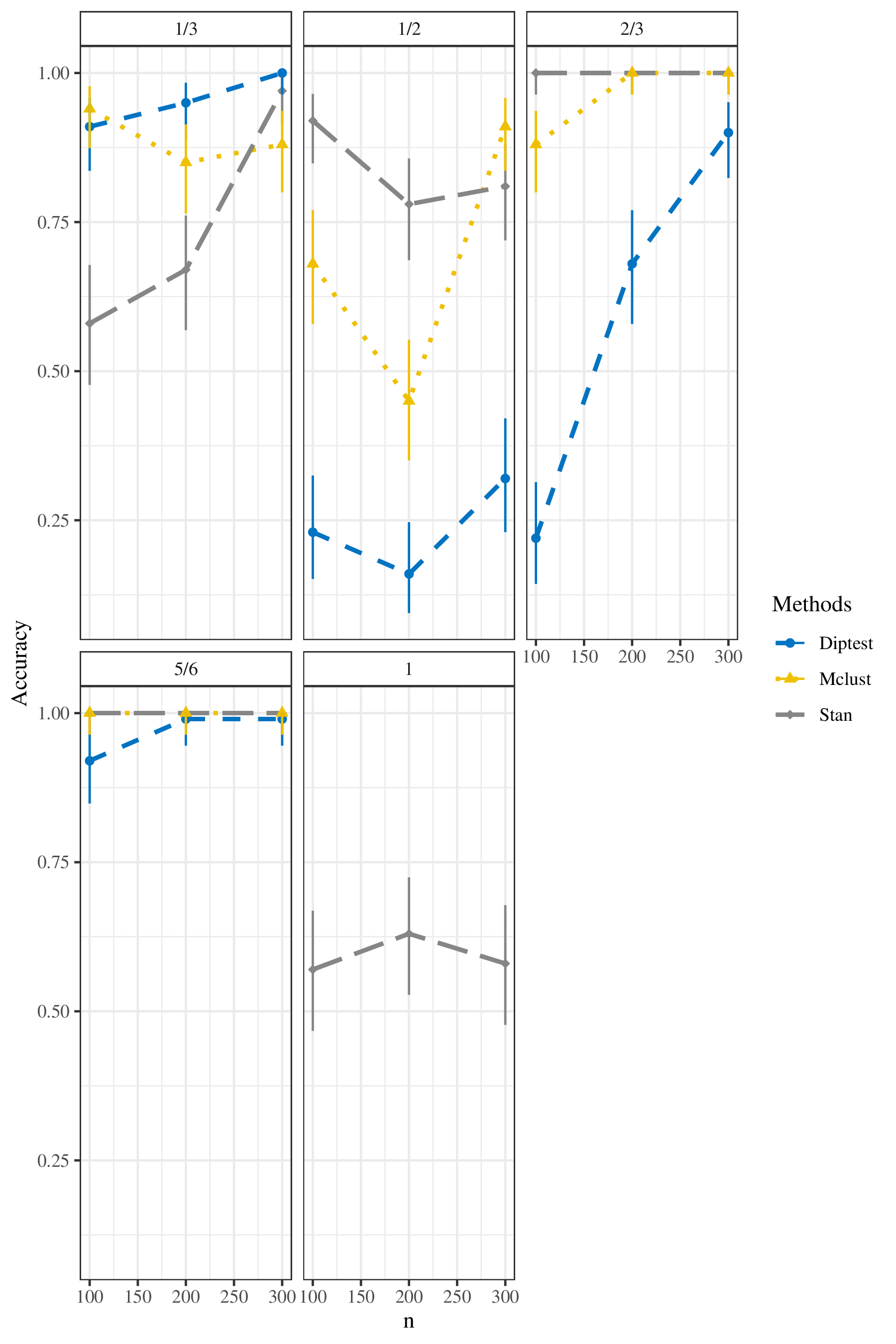 According to this plot, when the true value of \(\theta\) is
\(\frac{1}{3}\), the given data are from autopolyploidy. In this case,
Stan method performs worse than Mclust and dip test when the sample size
is small. When the sample size increases, the accuracy increases. For
dip test, the accuracy is higher than Stan when the sample size is
small. When the sample size increases, the accuracy also increases, and
when sample size = 300, the accuracy of dip test is 100%. For Mclust,
when the sample size is small, it has a good performance.
According to this plot, when the true value of \(\theta\) is
\(\frac{1}{3}\), the given data are from autopolyploidy. In this case,
Stan method performs worse than Mclust and dip test when the sample size
is small. When the sample size increases, the accuracy increases. For
dip test, the accuracy is higher than Stan when the sample size is
small. When the sample size increases, the accuracy also increases, and
when sample size = 300, the accuracy of dip test is 100%. For Mclust,
when the sample size is small, it has a good performance.
When the given data are from intermediate pairing behavior, the results are slightly different. When the true value of \(\theta\) is \(\frac{1}{2}\), Stan has the best performance when the sample size is 100 and 200. When the sample size is 300, Mclust also performs well. Dip test has the worst performance. When the true value of \(\theta\) is \(\frac{2}{3}\), Stan has the best performance, and the accuracy is 100%. Mclust’s accuracy can also achieve 100%, when the sample size is 200 and 300. Dip test still has the worst performance. With increasing sample size, accuracy of all three methods increase or stabilize. Similar to the previous situation, when the true value of \(\theta\) is \(\frac{5}{6}\), under this situation, the accuracy of both Stan and Mclust reaches 100%. When the sample size is 200 and 300, the accuracy of dip test can also reaches 100%. With increasing sample size, accuracy of all three methods increase or go stable.
When the given data are from allopolyploidy pairing behavior, the true value of \(\theta\) is 1. Only Stan can distinguish whether the given data are from allopolyploidy. When the sample size = 100, the accuracy is 57%, when the sample size = 200, the accuracy is 63%, and when the sample size = 300, the accuracy is 58%. The lower accuracy maybe result from the boundary issue. The \(\hat{\gamma} \in [0,1]\). When true \(\theta\) is 1, \(\hat\gamma\) is close on the boundary, and MLE theory breaks down here. We will work on this problem in the future.
| Group | True \(\theta\) | Sample Size | Method | Accuracy | Lower | Upper |
|---|---|---|---|---|---|---|
| 1 | \(\frac{1}{3}\) | 100 | Dip Test | 0.91 | 0.84 | 0.96 |
| 2 | \(\frac{1}{3}\) | 100 | Mclust | 0.94 | 0.87 | 0.98 |
| 3 | \(\frac{1}{3}\) | 100 | Stan | 0.58 | 0.48 | 0.68 |
| 4 | \(\frac{1}{3}\) | 200 | Dip Test | 0.95 | 0.89 | 0.98 |
| 5 | \(\frac{1}{3}\) | 200 | Mclust | 0.85 | 0.76 | 0.91 |
| 6 | \(\frac{1}{3}\) | 200 | Stan | 0.67 | 0.57 | 0.76 |
| 7 | \(\frac{1}{3}\) | 300 | Dip Test | 1.00 | 0.96 | 1.00 |
| 8 | \(\frac{1}{3}\) | 300 | Mclust | 0.88 | 0.80 | 0.94 |
| 9 | \(\frac{1}{3}\) | 300 | Stan | 0.97 | 0.91 | 0.99 |
| 10 | \(\frac{1}{2}\) | 100 | Dip Test | 0.23 | 0.15 | 0.32 |
| 11 | \(\frac{1}{2}\) | 100 | Mclust | 0.68 | 0.58 | 0.77 |
| 12 | \(\frac{1}{2}\) | 100 | Stan | 0.92 | 0.85 | 0.96 |
| 13 | \(\frac{1}{2}\) | 200 | Dip Test | 0.16 | 0.09 | 0.25 |
| 14 | \(\frac{1}{2}\) | 200 | Mclust | 0.45 | 0.35 | 0.55 |
| 15 | \(\frac{1}{2}\) | 200 | Stan | 0.78 | 0.69 | 0.86 |
| 16 | \(\frac{1}{2}\) | 300 | Dip Test | 0.32 | 0.23 | 0.42 |
| 17 | \(\frac{1}{2}\) | 300 | Mclust | 0.91 | 0.84 | 0.96 |
| 18 | \(\frac{1}{2}\) | 300 | Stan | 0.81 | 0.72 | 0.88 |
| 19 | \(\frac{2}{3}\) | 100 | Dip Test | 0.22 | 0.14 | 0.31 |
| 20 | \(\frac{2}{3}\) | 100 | Mclust | 0.88 | 0.80 | 0.94 |
| 21 | \(\frac{2}{3}\) | 100 | Stan | 1.00 | 0.96 | 1.00 |
| 22 | \(\frac{2}{3}\) | 200 | Dip Test | 0.68 | 0.58 | 0.77 |
| 23 | \(\frac{2}{3}\) | 200 | Mclust | 1.00 | 0.96 | 1.00 |
| 24 | \(\frac{2}{3}\) | 200 | Stan | 1.00 | 0.96 | 1.00 |
| 25 | \(\frac{2}{3}\) | 300 | Dip Test | 0.90 | 0.82 | 0.95 |
| 26 | \(\frac{2}{3}\) | 300 | Mclust | 1.00 | 0.96 | 1.00 |
| 27 | \(\frac{2}{3}\) | 300 | Stan | 1.00 | 0.96 | 1.00 |
| 28 | \(\frac{5}{6}\) | 100 | Dip Test | 0.92 | 0.85 | 0.96 |
| 29 | \(\frac{5}{6}\) | 100 | Mclust | 1.00 | 0.96 | 1.00 |
| 30 | \(\frac{5}{6}\) | 100 | Stan | 1.00 | 0.96 | 1.00 |
| 31 | \(\frac{5}{6}\) | 200 | Dip Test | 0.99 | 0.95 | 1.00 |
| 32 | \(\frac{5}{6}\) | 200 | Mclust | 1.00 | 0.96 | 1.00 |
| 33 | \(\frac{5}{6}\) | 200 | Stan | 1.00 | 0.96 | 1.00 |
| 34 | \(\frac{5}{6}\) | 300 | Dip Test | 0.99 | 0.95 | 1.00 |
| 35 | \(\frac{5}{6}\) | 300 | Mclust | 1.00 | 0.96 | 1.00 |
| 36 | \(\frac{5}{6}\) | 300 | Stan | 1.00 | 0.96 | 1.00 |
| 37 | 1 | 100 | Stan | 0.57 | 0.47 | 0.67 |
| 38 | 1 | 200 | Stan | 0.63 | 0.53 | 0.72 |
| 39 | 1 | 300 | Stan | 0.58 | 0.48 | 0.68 |
Conclusion
The pairing behavior of tetraploid species was discussed in this thesis and we described a way to directly estimate levels preferential pairing at individual loci using genotype data derived from NGS data. From the simulation study, we demonstrated that our model can estimate the preferential pairing parameter \(\gamma_{jk}\) accurately and distinguish between the three different pairing behaviors: autopolyploidy, intermediate, and allopolyploidy. After deriving \(\hat\gamma_j\) from MLE, we distinguish the ploidy type via model-based clustering. When the given data are from autopolyploids, our Stan method exhibits great performance, and when the sample size is large enough, the accuracy is high. For example, when the given data are from autopolyploids and sample size is 300, the accuracy is 97%. When the given data are from intermediate polyploids, through our Stan method, the highest accuracy is 100%. However, when the given data are from allopolyploids, MLE theory breaks down here, since the true value of \(\gamma\) is 1, but \(\gamma \in [0,1]\), which means that the estimate is on boundary. We will have more future work on this. Additionally, we also compared the Stan approach to that of Mclust and dip test to distinguish the ploidy type. These two methods can only distinguish whether the given data are from autopolyploidy. Compared with Stan method, the accuracy of dip test and Mclust is lower in most cases.
However, there are still a few weaknesses with our methods. By only exploring tetraploids, we excluded the consideration of higher ploidy levels. To avoid double reduction, the situation where one gamete receives two copies of part of the same parental hom(oe)olog, we only allow for bivalent pairing, and exclude quadrivalent pairing, which will lead to double reduction in some cases (Voorrips, Gort, and Vosman 2011; Bourke et al. 2017; Zheng et al. 2016).
Additionally, there are some statistical and computational limitations. For example, the number of iterations for simulation is relatively small, since we limited the number of simulation iterations for computational reasons. Additionally, as we mentioned above, MLE breaks down at the boundary, which leads to poor behavior when the given data are from allopolyploids. For future work, we will do more research to figure out the boundary issue (Marchand and Strawderman 2004; Zwiernik 2015).
Reference
Blischak, Paul D, Laura S Kubatko, and Andrea D Wolfe. 2018. “SNP Genotyping and Parameter Estimation in Polyploids Using Low-Coverage Sequencing Data.” Bioinformatics 34 (3): 407–15.
Bourke, Peter M., Paul Arens, Roeland E. Voorrips, G. Danny Esselink, Carole F. S. Koning-Boucoiran, Wendy P. C. van’t Westende, Tiago Santos Leonardo, et al. 2017. “Partial Preferential Chromosome Pairing Is Genotype Dependent in Tetraploid Rose.” The Plant Journal 90 (2): 330–43. https://doi.org/10.1111/tpj.13496.
Brent, Richard P. 1973. “Algorithms for Minimization Without Derivatives, Chap. 4.” Prentice-Hall Englewood Cliffs, NJ, USA.
Cao, Dachuang, Thomas C Osborn, and Rebecca W Doerge. 2004. “Correct Estimation of Preferential Chromosome Pairing in Autotetraploids.” Genome Research 14 (3): 459–62.
Casella, G., and R. L. Berger. 2002. Statistical Inference. Duxbury Advanced Series in Statistics and Decision Sciences. Thomson Learning. https://books.google.com/books?id=0x\_vAAAAMAAJ.
Clark, Lindsay V, Alexander E Lipka, and Erik J Sacks. 2019. “PolyRAD: Genotype Calling with Uncertainty from Sequencing Data in Polyploids and Diploids.” G3: Genes, Genomes, Genetics 9 (3): 663–73.
Coward, Jermaine, and Angus Harding. 2014. “Size Does Matter: Why Polyploid Tumor Cells Are Critical Drug Targets in the War on Cancer.” Frontiers in Oncology 4: 123.
Gerard, David, and Luís Felipe Ventorim Ferrão. 2019. “Priors for genotyping polyploids.” Bioinformatics 36 (6): 1795–1800. https://doi.org/10.1093/bioinformatics/btz852.
Gerard, David, Luís Felipe Ventorim Ferrão, Antonio Augusto Franco Garcia, and Matthew Stephens. 2018. “Genotyping Polyploids from Messy Sequencing Data.” Genetics 210 (3): 789–807. https://doi.org/10.1534/genetics.118.301468.
Hartigan, John A, Pamela M Hartigan, and others. 1985. “The Dip Test of Unimodality.” The Annals of Statistics 13 (1): 70–84.
Hilu, K. W. 1993. “Polyploidy and the Evolution of Domesticated Plants.” American Journal of Botany 80 (12): 1494–9. http://www.jstor.org/stable/2445679.
Joly, Simon, Julian Starr, Walter Lewis, and Anne Bruneau. 2006. “Polyploid and Hybrid Evolution in Roses East of the Rocky Mountains.” American Journal of Botany 93 (March): 412–25. https://doi.org/10.3732/ajb.93.3.412.
Maechler, Martin. 2016. Diptest: Hartigan’s Dip Test Statistic for Unimodality - Corrected. https://CRAN.R-project.org/package=diptest.
Marchand, Eric, and William E. Strawderman. 2004. “Estimation in Restricted Parameter Spaces: A Review.” Lecture Notes-Monograph Series 45: 21–44. http://www.jstor.org/stable/4356296.
Mason, Annaliese S. 2017. Polyploidy and Hybridization for Crop Improvement. CRC Press.
Otto, Sarah P, and Jeannette Whitton. 2000. “Polyploid Incidence and Evolution.” Annual Review of Genetics 34 (1): 401–37.
Scrucca, Luca, Michael Fop, T Brendan Murphy, and Adrian E Raftery. 2016. “Mclust 5: Clustering, Classification and Density Estimation Using Gaussian Finite Mixture Models.” The R Journal 8 (1): 289.
Stan Development Team. 2018. “Stan Modeling Language Users Guide and Reference Manual, Version 2.18.0.” http://mc-stan.org/.
———. 2020. “RStan: The R Interface to Stan.” http://mc-stan.org/.
Sybenga, J. 1994. “Preferential Pairing Estimates from Multivalent Frequencies in Tetraploids.” Genome 37 (6): 1045–55. https://doi.org/10.1139/g94-149.
Voorrips, Roeland E, Gerrit Gort, and Ben Vosman. 2011. “Genotype Calling in Tetraploid Species from Bi-Allelic Marker Data Using Mixture Models.” BMC Bioinformatics 12 (1): 172.
Voorrips, Roeland, and Chris Maliepaard. 2012. “The Simulation of Meiosis in Diploid and Tetraploid Organisms Using Various Genetic Models.” BMC Bioinformatics 13 (September): 248. https://doi.org/10.1186/1471-2105-13-248.
Wendel, Jonathan F. 2000. “Genome Evolution in Polyploids.” In Plant Molecular Evolution, 225–49. Springer.
Wu, Rongling, Maria Gallo-Meagher, Ramon C Littell, and Zhao-Bang Zeng. 2001. “A General Polyploid Model for Analyzing Gene Segregation in Outcrossing Tetraploid Species.” Genetics 159 (2): 869–82.
Zheng, Chaozhi, Roeland E Voorrips, Johannes Jansen, Christine A Hackett, Julie Ho, and Marco CAM Bink. 2016. “Probabilistic Multilocus Haplotype Reconstruction in Outcrossing Tetraploids.” Genetics 203 (1): 119–31.
Zwiernik, P. 2015. Semialgebraic Statistics and Latent Tree Models. Chapman & Hall/Crc Monographs on Statistics & Applied Probability. CRC Press. https://books.google.com/books?id=YdWYCgAAQBAJ.
Ruiqi Sun
My research interests include data science and artificial intelligence.